Example

This page goes over a simple usage of the library. We will analyse a chess matches dataset to determine the effect of blunders on centipawn loss.

Analysing the problem

First, some chess terminology:

Blunders are moves that are considered unforgivable errors

Centipawn Loss is a measure of how much of a disadvantage the play is in: 100 centipawn equals 1 pawn.

Rating is a measure of how skilled a player is, for matchmaking purposes.

The dataset contains data regarding white’s and black’s number of blunders, average centipawn loss and rating. It also contains other features, but we will ignore them for simplicity sake.

Our task is to determine the effect of blunders on centipawn loss: in short, just how many pawns you lose by making blunders.

import numpy as np
import pandas as pd
import seaborn as sns

df = pd.read_csv('chess.csv')
df = df.drop(["Unnamed: 0", "Game ID", "Opening Ply", "Opening ECO", "White's Number of Inaccuracies", "White's Number of Mistakes", "Black's Number of Inaccuracies", "Black's Number of Mistakes"], axis=1)

As a sanity check, we will first take a look at the relation between white’s number of blunders and black centipawn loss. Common sense makes would makes us think that the causal relationship there would be small or negative, since white’s mistakes should not impact black’s ability to play the game.

Plotting these variables for visualization:

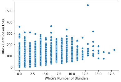
The plot reveals a surprising association: the more blunder’s white makes, the worst black plays.

This very likely happens because matchmaking assures that bad players meet other bad players, and good players meet good players. So if white is making a small amount of mistakes, odds are he is good at the game and is facing opponents who also are. This is an example of common cause bias, and it can be avoided by using a causal inference model that controls for matchmaking in some way. To learn more about that, check out causal graphs.

In this case, we will control for white’s and black’s rating, as well as black’s number of blunders. This way, we will hopefully compare only players with similar skill. The model we are going to use for that is the SLearner.

Applying the model

Now, to simplify the problem we will make our treatment data binary. This means we will only consider two situations: you either make a lot of blunders, or you dont.

treatment_col = "White's Number of Blunders"
treatment = (df[treatment_col] >= df[treatment_col].mean()).astype(int)

We then create our model. We are going to use the pycausal_explorer.linear._linear_models, a meta learner, using sklearn’s causal forests as the predictor.

from pycausal_explorer.meta import SingleLearnerRegressor
from sklearn.ensemble import RandomForestRegressor

learner = SingleLearnerRegressor(RandomForestRegressor())

We will then fit our model to the data, and predict the treatment effect

learner.fit(df[["Black Rating", "White Rating", "Black's Number of Blunders"]], df["Black Centi-pawn Loss"], treatment=treatment)
resB = learner.predict_ite(df[["Black Rating", "White Rating", "Black's Number of Blunders"]])
print("Effect of white's blunders on black's loss: ", resB.mean())

Effect of white's blunders on black's loss:  -1.4069125492747534

As expected, the effect is pretty small. It’s also negative, which makes sense: If white is playing poorly, black should find less opportunities to misplay. So let’s move on to the effect on white’s centipawn loss

learner.fit(df[["Black Rating", "White Rating", "Black's Number of Blunders"]], df["White Centi-pawn Loss"], treatment=treatment)
resB = learner.predict_ite(df[["Black Rating", "White Rating", "Black's Number of Blunders"]])
print("Effect of white's blunders on whitw's loss: ", resB.mean())

Effect of white's blunders on white's loss:   41.63210605667355

We can see it’s somewhat big, as it should be.

By now you should have an idea of how this library’s work. If you want to decide which model to use, check out out Model Guide. If you want to know every model we have, we also have a Model List.