Model Guide

In this section, we outline each model strong and weak points and recommended use cases.

Meta learners

Meta learners rely on machine learning models that predict outcome. Their performance is tied to how well the provided model can learn the outcome function. [1]

They perform poorly when the outcome is hard to predict, such as when there are too many covariables or the generating function is too complex. [2] They are also strongly affected by regularization.

Bellow we outline each one. Overall, unless the SLearner’s bias towards zero is desirable, the XLearner has the best convergence rate.

SLearner

The Slearner treats the treatment indicator like any other predictor. [1]. It is often biased towards 0, and is more accurate when treatment effect is often 0 or close to 0.

TLearner

The Tlearner does not combine the treated and control groups, but instead creates a model for each. It’s less data efficient, but performs better when both groups behave very differently. [1]

XLearner

The XLearner applies a machine learning model to predict treatment effect, on top of the ones to predict treatment and control groups. [1] It performs better all around, and particularly well when there are many more entries in one group than in the other. [2]

Double / Debiased learner

The Double learner, also known as Debiased learner, is a meta learner that aims to discover traits of a dataset’s data generating function rather than of the outcome itself.

By training a leaner to predict the impact the covariables have on the outcome, and likewise for the treatment, the model can subtract said impact to ‘debias’ the data, allowing for more direct inference of the relation between outcome and treatment.

It performs well even when there are many covariables [5] , and can avoid overfitting fairly well by means of K fold validation. [7]

Double ML linear

Linear version. Should be used when treatment effect is linear, and the treatment variable is continuous. Assumes the data is distributed according to the model:

$Y = D \theta_0 + g_0(X) + \zeta$

$D = m_0(X) + V$

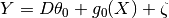
where

Y is the outcome
D is the treatment
X are the covariables controled for
$\zeta$ and $V$ are errors.
$\theta_0$ is the treatment effect
$g_0$ is the function that describes the impact of X on Y
$m_0$ is the function that describes the impact of X on D

The functions $g_0$ and $m_0$ are estimated by learners provided by the user.

Double ML binary

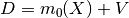
Binary treatment version. Should be used when treatment is a binary variable. Assumes the data is distributed according to the model:

$Y = g_0(D, X) + U$

$D = m_0(X) + V$

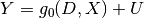
where

Y is the outcome
D is the treatment
X are the covariables controled for
$U$ and $V$ are errors.
$g_0$ is the function that describes the impact of X on Y
$m_0$ is the function that describes the impact of X on D

The functions $g_0$ and $m_0$ are estimated by learners provided by the user.

Linear Learners

Linear learners are versions of the SLearner restricted to the LinearRegressor and LogisticRegressor models. They are implemented mostly for educational and illustrative purposes.

Causal Forests

The causal forests model makes use of two different models: a random forest to reduce noise, and a KNN to match the feature to the nearby features that went trough treatment, and the ones that did not. [5]

Causal forests are very good at predicting complex treatment effects, that vary strongly and non-linearly between features. They can perform well even the outcome function is very complex, since they do not need to estimate it. [3] [4]

Nearest Neighbor

The nearest neighbors model aims to find similar data points to the one being analysed. It generally performs worse than the causal forests model.

IPTW

The Inverse Probability Treatment Weighting (IPTW) model will use the propensity score, which is the likelihood every feature has of being treated, as a replacement for all the covariables. As a result the treatment effect estimation is simplified.